> clust.coeff<-function(matrix){
+ n<-nrow(matrix)
+ output<-rep(0,n)
+ for(i in 1:n){
+ m<-sum(matrix[i,])
+ output[i]<-
+ sum(t(matrix * matrix[i,])*matrix[i,])/(m*(m-1))
+ }
+ output[which(output=="NaN")]<-0
+ output
+ }

> A<-matrix(c(
+ 0,1,1,1,1,0,0,0,0,
+ 1,0,1,1,1,1,0,0,0,
+ 1,1,0,1,0,0,1,0,0,
+ 1,1,1,0,0,0,0,1,1,
+ 1,1,0,0,0,0,0,0,0,
+ 0,1,0,0,0,0,0,0,0,
+ 0,0,1,0,0,0,0,0,0,
+ 0,0,0,1,0,0,0,0,0,
+ 0,0,0,1,0,0,0,0,0),
+ nrow = 9)

> clust.coeff(A)
[1] 0.6666667 0.4000000 0.5000000 0.3000000 1.0000000 0.0000000 0.0000000
[8] 0.0000000 0.0000000

> mean(clust.coeff(A))
[1] 0.3185185

 
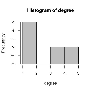
> library(sna)
degree <- degree(A)/2
hist(degree, col = "grey")

 
> rgraph(100,tprob=0.01,mode="graph")
       [,1] [,2] [,3] [,4] [,5] [,6] [,7] [,8] [,9] [,10] [,11] [,12] [,13]
  [1,]    0    0    0    0    0    0    0    0    0     0     0     0     0
  [2,]    0    0    1    0    0    0    0    0    0     0     0     0     0
  [3,]    0    1    0    0    0    0    0    0    0     0     0     0     0
  [4,]    0    0    0    0    0    0    0    0    0     0     0     0     0
  [5,]    0    0    0    0    0    0    0    0    0     0     0     0     0

略

 
> erdos.renyi.game(100,p=0.01)
Vertices: 100 
Edges: 51 
Directed: FALSE 
Edges:
             
[0]   4 -- 22
[1]   2 -- 23
[2]   6 -- 25
[3]   6 -- 27
[4]   0 -- 29
[5]   9 -- 30
[6]   9 -- 35

略

 
> random.graph.game(100, p = 0.01)
Vertices: 100 
Edges: 35 
Directed: FALSE 
Edges:
             
[0]   1 --  7
[1]   7 --  8
[2]  15 -- 25
[3]  32 -- 40
[4]  19 -- 41
[5]   8 -- 44

 
> rg <- rgraph(100, tprob = 0.05, mode = "graph")
> distance <- geodist(rg)$gdist
> mean(distance[-c(which(distance == Inf), which(distance == 0))])
[1] 3.150484
> mean(clust.coeff(rg))
[1] 0.0345
> degree <- degree(rg)/2
> hist(degree, col = "grey")

 
#レギュラーグラフ作成関数
regular.g <- function(n,k) {
  reg <- matrix(0,n,n)
  for (i in 1:n){
    for (j in 1:k){
      if (i+j <= n) 
        reg[i,i+j] <- 1
      else 
        reg[i,i+j-n] <- 1
    }
  }
(reg <- symmetrize(reg))
}

#スモールワールド・シミュレーション
g <- regular.g(100,4)
Clustering <- 1:101
Distance <- 1:101
p <- seq(0,1,by = 0.01)
for (i in 1:101) {
  clust <- 1:20
  dist <- 1:20
  for (j in 1:20){ 
    rew.g <- rewire.ws(g, p[i])[1,,]
    clust[j] <- mean(clust.coeff(rew.g))
    d <- geodist(rew.g)$gdist
    dist[j] <- mean(d[-c(which(d == Inf),which(d == 0))])
  }
  Clustering[i] <- mean(clust)
  Distance[i] <- mean(dist)
}

x <- p; y <- Clustering
plot(x, y, xlab ="p", ylab = "Clustering Coefficient")

x <- p; y <- Distance
plot(x, y, xlab ="p", ylab = "Average Distance")

x <- p
y <- matrix(c(Clustering/Clustering[1],Distance/Distance[1]),101,2)
matplot(x, y, log = "x", pch = c(1,2), xlab ="p", ylab = "", col = "black")
legend(locator(1), pch = c(1,2), 
c("clustering coefficient","average distance"))

 
g <- barabasi.game(10000, m = 2, directed = FALSE)
dd <- degree.distribution(g)
plot(dd,log ="x", xlab = "degree", ylab = "proportion")
plot(dd,log ="xy", xlab = "degree", ylab = "proportion")
average.path.length(g)

clust <- transitivity(g,type ="local")
clust[which(clust == "NaN")] <- 0
mean(clust)

 
> library("igraph")
> graph2<-barabasi.game(1000,power=1)
> write.graph(graph2,"table2.txt","edgelist")