


多変量時系列解析に関しては、最も広く知られているのはベクトル自己回帰 (VAR: Vector AutoRegressive) モデルである。
多変量時系列の標本データを
とすると(誘導型)VARモデルは次のように定義される。
モデルの中の係数A1,A2,…,Apは行列、 残差Etはベクトルである。
VARモデルを推定するためには、2種類の方法がある。 パッケージtseriesを利用するか、VARモデル専用のパッケージである、varsを利用するかである。
1)パッケージtseriesの利用
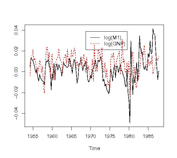
1つ目は、tseriesを用いて、その中に入っているarima関数または、ar関数を用いる方法である。 ここではパッケージtseriesの中に用意されている、 1954年の第1四半期から1987年第4四半期までのアメリカの4 変量の経済時系列データUSeconomicの中の先頭の2変量を用いる。 第1変量はlog(GNP)=実質GNP の対数値(季調済み)、第2変量はlog(M1)=実質M1 の対数値(季調済み)である。 データにはトレンドがあるので、1階差分を取って用いる。
> library(tseries); > data(USeconomic) > USe.d<-diff(USeconomic[,1:2]) > ts.plot(USe.d,lty=c(1,2),col=c(1,2)) > legend(locator(1),c(colnames(USe.d)[1],colnames(USe.d)[2]),lty=c(1,2),col=c(1,2)) |
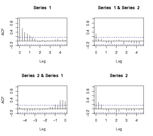
自己相関は、単変量の場合と同じく次のように関数acfで求めることができる。
> acf(USe.d, na.action=na.pass) |
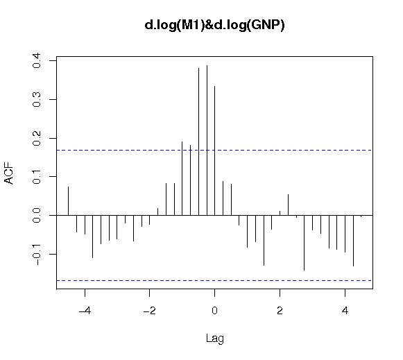
また、相互相関は、次のように関数ccfで求めることができる。
>ccf(USe.d[,1],USe.d[,2],main="d.log(M1) & d.log(GNP)") |
関数arを用いたVARモデルを当てはめる例を次に示す。 関数arでは、引数aic=TRUEで計算すると自動的に最適な次数の推定値に基づいて結果を返す。 ここでは、返す結果とモデルの対応関係を説明するため、 次のように強制的にVAR(2)モデル(必ずしも最適なケースではない)の推定値を求める。
> (USe.ar<-ar(USe.d,order.max=2,aic=F))

Call:
ar(x = USe.d, aic = F, order.max = 2)

$ar
, , 1

       [,1]    [,2]
[1,] 0.5446 -0.1888
[2,] 0.1981  0.1295

, , 2

       [,1]    [,2]
[1,] 0.1231 0.04513
[2,] 0.1371 0.07110


$var.pred
          [,1]      [,2]
[1,] 1.063e-04 1.506e-05
[2,] 1.506e-05 8.494e-05
|
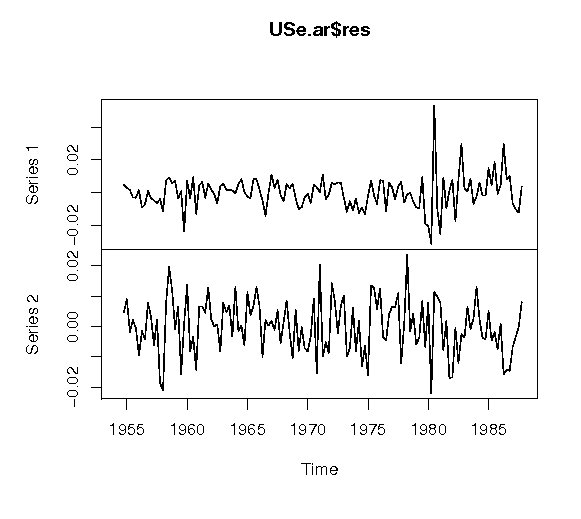
返された結果を用いた2変量のモデルを次に示す。
式の中のMはlog(M1)の1階差分値で、Mはlog(GNP)の1階差分値である。残差のプロットを次に示す。
> plot(USe.ar$res)) |
作成したモデルの予測値は次のように求めることができる。 ただし、現在のバージョンでは多変量時系列の予測値の推定標準誤差は計算できないので、se.fit=Fにする。
> USe.f<-predict(USe.ar,n.ahead=12,se.fit=F) |
2)パッケージvarsの利用
> library(vars)

> v1<-VAR(USe.d,p=1,type="const")

> summary(v1)

VAR Estimation Results:
=========================
Endogenous variables: log.M1., log.GNP.
Deterministic variables: const
Sample size: 134
Log Likelihood: 865.363
Roots of the characteristic polynomial:
0.4715 0.323
Call:
VAR(y = USe.d, p = 1, type = "const")


Estimation results for equation log.M1.:
========================================
log.M1. = log.M1..l1 + log.GNP..l1 + const

             Estimate Std. Error t value Pr(>|t|)
log.M1..l1   0.605185   0.075740   7.990 6.09e-13 ***
log.GNP..l1 -0.142638   0.093215  -1.530    0.128
const        0.002032   0.001112   1.827    0.070 .
---
Signif. codes:  0 ‘***’ 0.001 ‘**’ 0.01 ‘*’ 0.05 ‘.’ 0.1 ‘ ’ 1


Residual standard error: 0.01033 on 131 degrees of freedom
Multiple R-Squared: 0.3327,     Adjusted R-squared: 0.3225
F-statistic: 32.66 on 2 and 131 DF,  p-value: 3.103e-12


Estimation results for equation log.GNP.:
=========================================
log.GNP. = log.M1..l1 + log.GNP..l1 + const

             Estimate Std. Error t value Pr(>|t|)
log.M1..l1  0.2644613  0.0678459   3.898 0.000154 ***
log.GNP..l1 0.1893458  0.0834998   2.268 0.024990 *
const       0.0055944  0.0009962   5.616 1.12e-07 ***
---
Signif. codes:  0 ‘***’ 0.001 ‘**’ 0.01 ‘*’ 0.05 ‘.’ 0.1 ‘ ’ 1


Residual standard error: 0.00925 on 131 degrees of freedom
Multiple R-Squared: 0.1842,     Adjusted R-squared: 0.1717
F-statistic: 14.79 on 2 and 131 DF,  p-value: 1.622e-06


Covariance matrix of residuals:
           log.M1.  log.GNP.
log.M1.  0.0001066 1.750e-05
log.GNP. 0.0000175 8.557e-05

Correlation matrix of residuals:
         log.M1. log.GNP.
log.M1.   1.0000   0.1832
log.GNP.  0.1832   1.0000
|
構造型VARモデルの推定
Aが非特異であるならば、両辺に左より逆行列をかけることにより、 誘導型VARモデルに変換する事ができる。
Granger因果性とインパルス応答関数
> varset<-read.table("varset.txt",header=T)
> ci<-varset[,2]
> cpi<-varset[,3]
> call<-varset[,4]
> lci<-100*log(ci)
> lcpi<-100*log(cpi)
> dci<-100*diff(log(ci))
> set<-data.frame(lci,lcpi,call)
> v1<-VAR(set,p=1,type="const")
> summary(v1)

VAR Estimation Results:
=========================
Endogenous variables: lci, lcpi, call
Deterministic variables: const
Sample size: 115
Log Likelihood: -123.391
Roots of the characteristic polynomial:
0.9506 0.9506 0.9221
Call:
VAR(y = set, p = 1, type = "const")


Estimation results for equation lci:
====================================
lci = lci.l1 + lcpi.l1 + call.l1 + const

         Estimate Std. Error t value Pr(>|t|)
lci.l1    0.97007    0.01527  63.535  < 2e-16 ***
lcpi.l1  -0.30549    0.11070  -2.760  0.00677 **
call.l1  -0.44240    0.10051  -4.401 2.48e-05 ***
const   155.23398   51.46163   3.016  0.00317 **
---
Signif. codes:  0 ‘***’ 0.001 ‘**’ 0.01 ‘*’ 0.05 ‘.’ 0.1 ‘ ’ 1


Residual standard error: 0.8835 on 111 degrees of freedom
Multiple R-Squared: 0.9734,     Adjusted R-squared: 0.9727
F-statistic:  1354 on 3 and 111 DF,  p-value: < 2.2e-16


Estimation results for equation lcpi:
=====================================
lcpi = lci.l1 + lcpi.l1 + call.l1 + const

         Estimate Std. Error t value Pr(>|t|)
lci.l1   0.004363   0.005809   0.751   0.4541
lcpi.l1  0.890746   0.042112  21.152   <2e-16 ***
call.l1 -0.061823   0.038239  -1.617   0.1088
const   48.559615  19.577614   2.480   0.0146 *
---
Signif. codes:  0 ‘***’ 0.001 ‘**’ 0.01 ‘*’ 0.05 ‘.’ 0.1 ‘ ’ 1


Residual standard error: 0.3361 on 111 degrees of freedom
Multiple R-Squared: 0.9623,     Adjusted R-squared: 0.9613
F-statistic: 945.4 on 3 and 111 DF,  p-value: < 2.2e-16


Estimation results for equation call:
=====================================
call = lci.l1 + lcpi.l1 + call.l1 + const

          Estimate Std. Error t value Pr(>|t|)
lci.l1   0.0006135  0.0025719   0.239    0.812
lcpi.l1  0.0036994  0.0186468   0.198    0.843
call.l1  0.9623283  0.0169317  56.836   <2e-16 ***
const   -1.9855258  8.6687166  -0.229    0.819
---
Signif. codes:  0 ‘***’ 0.001 ‘**’ 0.01 ‘*’ 0.05 ‘.’ 0.1 ‘ ’ 1


Residual standard error: 0.1488 on 111 degrees of freedom
Multiple R-Squared: 0.9939,     Adjusted R-squared: 0.9937
F-statistic:  5992 on 3 and 111 DF,  p-value: < 2.2e-16


Covariance matrix of residuals:
           lci      lcpi      call
lci   0.780550 -0.028677  0.006348
lcpi -0.028677  0.112967 -0.005527
call  0.006348 -0.005527  0.022148

Correlation matrix of residuals:
          lci     lcpi     call
lci   1.00000 -0.09657  0.04828
lcpi -0.09657  1.00000 -0.11049
call  0.04828 -0.11049  1.00000


> causality(v1,cause="call")
$Granger

        Granger causality H0: call do not Granger-cause lci lcpi

data:  VAR object v1
F-Test = 11.7903, df1 = 2, df2 = 333, p-value = 1.129e-05


$Instant

        H0: No instantaneous causality between: call and lci lcpi

data:  VAR object v1
Chi-squared = 1.547, df = 2, p-value = 0.4614
|
インパルス反応関数
> impulse<-irf(v1,impulse="call",response=c("lci","lcpi","call"),boot=TRUE)
> plot(impulse)
|
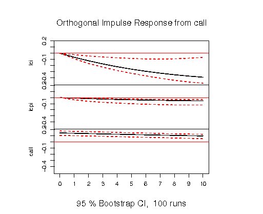
実線がインパルス応答関数であり、破線はブートストラップ法により求めた95%信頼区間である。 一番上の図は、callのインパルスに対して、lciは遅れて有意に負の反応を示す。 同様に、callのインパルスに対して、lcpiも有意に負の反応をしている。 一方、callのインパルスに対して、call自身は、始めは正の反応をしているものの、 その影響は次第に薄れていく事を示している。
共和分
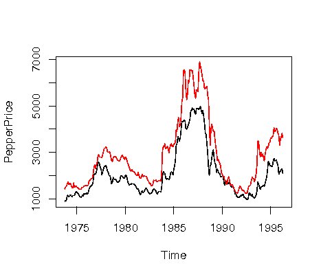
短期的には異なることもあるが、長期的には同じ動きをするような2つ以上のデータがある場合、 共和分関係にあるといわれている。 まず共和分関係にあるかどうかを調べる関数として、po.test()がある。
> library(AER)

> data("PepperPrice")
> plot(PepperPrice,plot.type="single",col=1:2)

> library(tseries)
> po.test(log(PepperPrice))

        Phillips-Ouliaris Cointegration Test

data:  log(PepperPrice)
Phillips-Ouliaris demeaned = -24.0987, Truncation lag parameter = 2,
p-value = 0.02404
|
これから統計量が負であり、絶対値が十分大きいことから, この2つのデータは共和分関係であることを示している。 詳しくはHamilton, J.W.「時系列解析〈下〉非定常/応用定常過程編」
この関係にある場合には、Grangerの表現定理(Granger and Engle(1987))から誤差修正モデル(Error Correction Model)に帰着することが知られている。これを調べるにはco.jo()の関数が知られている。
> library(urca)
> pepper_jo<-ca.jo(log(PepperPrice),ecdet="const",type="trace")
> summary(pepper_jo)

######################
# Johansen-Procedure #
######################

Test type: trace statistic , without linear trend and constant in cointegration

Eigenvalues (lambda):
[1] 4.931953e-02 1.350807e-02 2.081668e-17

Values of teststatistic and critical values of test:

          test 10pct  5pct  1pct
r <= 1 |  3.66  7.52  9.24 12.97
r = 0  | 17.26 17.85 19.96 24.60

Eigenvectors, normalised to first column:
(These are the cointegration relations)

           black.l2 white.l2   constant
black.l2  1.0000000  1.00000   1.000000
white.l2 -0.8892307 -5.09942   2.280911
constant -0.5569943 33.02742 -20.032441

Weights W:
(This is the loading matrix)

           black.l2    white.l2     constant
black.d -0.07472300 0.002453210 2.697730e-17
white.d  0.02015611 0.003537005 3.401573e-18
|
Back to R